Introduction to data.table in R

One of the most exciting packages in the R universe is data.table. This package allows you to create data.table objects as an alternative to data.frame. The benefit of using data.table is the speed and efficiency when working with large datasets, and a concise syntax that can be really easy to use once you get used to it.

Load data.table package and dataset

Lets first start with installing and loading the package. For this demonstration we will use the iris dataset that is preinstalled in R.

install.packages("data.table")
library(data.table)

data = setDT(copy(iris)) 
#note we have to create a copy because iris is built-in to R and thus not modifiable

In this case we didn’t import our data from a csv file, but if you have a large dataset that you need to import, the fread() function from data.table allows for extremely quick importing of data from either a csv file or a URL.

Also, here we converted an existing data frame to a data table object using setDT(). We could also use as.data.frame() for an existing object, or create our own data table by inputting data using data.table()

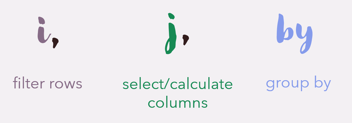
Data Table Syntax

The main syntax that data table uses is the DT[i, j, by]

This syntax allows for data to be manipulated extremely easily and in only one line of code! It may seem pretty foreign, so lets go through some explanations and examples.

Filter rows

Let’s say we only want the 15th row of our dataset. Or only data for flowers of the versicolor species. Or only data for the versicolor species with a sepal width less than 3. This is all easy to do in the “i” part of a data table.

#15th row

row_15 <- data[15]
row_15

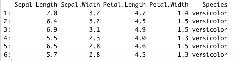
# versicolor species
versicolor <- data[Species == "versicolor"]
head(versicolor)

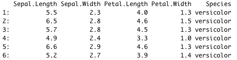
#versicolor species with a sepal width less than 3
versicolor_sepal3 <- data[Species == "versicolor" & Sepal.Width < 3]
head(versicolor_sepal3)

Other special operators include %in% and %between%

setosa_virginica <- data[Species %in% c("setosa", "virginica")]

pl_1.2_1.6 <- data[Petal.Length %between% c(1.2, 1.6)]

Working with columns

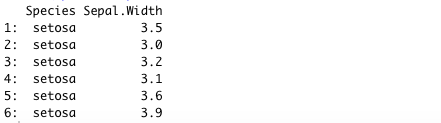
Let say you want to filter your dataset to contain all rows, but only the Species and Sepal Width columns. Note that you will leave the i section empty by just adding a comma before the j section.

species_sepalw <- data[, c("Species", "Sepal.Width")]

#an alternate way of writing a list in data.table is by using .() 
species_sepalw <- data[, .(Species, Sepal.Width)]
head(species_sepalw)

It is also easy to do computations on columns in data.table. Let’s find the median sepal width

median_sw <- data[, median(Sepal.Width)]
median_sw 

The := Operator: Creating New Columns

Using the “:=” operator in the j section allows you to create new columns using existing ones. When creating columns by reference, you don’t have to assign the result to a new object, because the column will be directly added to the current data table. For example, let’s compute sepal area (length x width)

data[, Sepal.Area := Sepal.Length * Sepal.Width]
head(data)

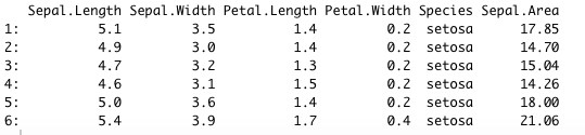
Notice how the new column name is on the left of the operator, and the operation is on the right.

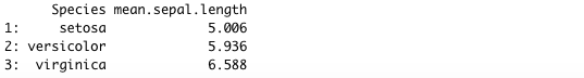
Group by variables

We can use the last section to group variables using “by”. For example, we can get the mean Sepal length by species.

mean_by_species <- data[, .(mean.sepal.length = mean(Sepal.Length)), by = Species]
mean_by_species

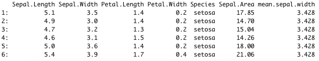
You can also create a new column by using the := operator, that is grouped by a variable (or multiple variables).

data[, mean.sepal.width := mean(Sepal.Width), by = Species]

The .N special symbol

Using the .N symbol means the number of rows present. This can function similarly to nrows(). For example, here we can get the number of rows where the sepal width is less than 3 and sepal length is less than 5.

less_3_5 <- data[Sepal.Width < 3 & Sepal.Length < 5, .N]
less_3_5

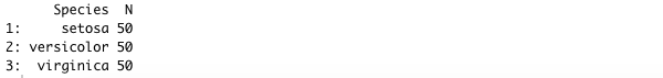
.N becomes really useful when you want to also use “by”. For example let’s get the number of observations per species.

obs <- data[, .N, by = Species]
obs

There are lots of other features of data.table that make it useful to use for data manipulation, but here I have gone over the basics and the operations that I use most often. Notice how easy it is to manipulate tables and combine multiple operations in only one line of code! If you are looking for more resources on using data.table you can:

1. Visit the CRAN
2. Complete a datacamp tutorial. Here is one called Data Manipulation with data.table in R
3. Check out the CRAN Vignette called Introduction to data.table

Happy analyzing!